Continuous Intraday Demo: Rolling Intrinsic Policy

Introduction

This example demonstrates how to use RTC-Tools to optimise a BESS for continuous intraday trading using the rolling intrinsic policy. The optimisation makes trading decisions based on the current orderbook state with a receding horizon, allocating power across multiple price levels in the bid and ask orderbooks.

The rolling intrinsic policy is a widely-used approach for real-time battery trading that optimizes over a receding horizon window, making decisions based on current market conditions.

Problem Formulation

Mathematical Model

The continuous intraday trading problem extends the basic BESS optimization with orderbook-aware trading:

Objective Function:

\[\max \sum_{t} \left( \sum_{i=1}^{N} P_{discharge,i}^{new}(t) \cdot \pi_{bid,i}(t) - \sum_{i=1}^{N} P_{charge,i}^{new}(t) \cdot \pi_{ask,i}(t) - \lambda_{tx} \cdot (P_{charge}^{new}(t) + P_{discharge}^{new}(t)) - \lambda_{cyc} \cdot (P_{charge}^{new}(t) + P_{discharge}^{new}(t)) \right)\]

Where:

\(P_{discharge,i}^{new}(t)\) = New power sold at bid level \(i\) (intraday trades only)
\(P_{charge,i}^{new}(t)\) = New power bought at ask level \(i\) (intraday trades only)
\(\pi_{bid,i}(t)\) = Bid price at level \(i\) (descending order)
\(\pi_{ask,i}(t)\) = Ask price at level \(i\) (ascending order)
\(N\) = Number of orderbook levels (default: 10)
\(\lambda_{tx}\) = Transaction cost per MWh traded
\(\lambda_{cyc}\) = Cycling penalty factor (requires tuning based on market conditions)

Power Allocation Constraints:

\[P_{discharge}^{new}(t) = \sum_{i=1}^{N} P_{discharge,i}^{new}(t)\]

\[P_{charge}^{new}(t) = \sum_{i=1}^{N} P_{charge,i}^{new}(t)\]

\[0 \leq P_{discharge,i}^{new}(t) \leq V_{bid,i}(t) \quad \forall i\]

\[0 \leq P_{charge,i}^{new}(t) \leq V_{ask,i}(t) \quad \forall i\]

Where:

\(V_{bid,i}(t)\) = Available volume at bid level \(i\)
\(V_{ask,i}(t)\) = Available volume at ask level \(i\)

Committed Position Integration:

The model accounts for committed positions from day ahead and prior intraday trades:

\[P_{net}(t) = P_{committed}(t) + P_{discharge}^{new}(t) - P_{charge}^{new}(t)\]

Where:

\(P_{committed}(t)\) = Net committed power from prior trades (positive=discharge, negative=charge)
\(P_{net}(t)\) = Total net power position after netting committed and new intraday trades

Splitting Constraint:

The net power is decomposed into non-negative charge and discharge components:

\[P_{net}(t) = P_{discharge}^{total}(t) - P_{charge}^{total}(t)\]

\[P_{discharge}^{total}(t) \geq 0, \quad P_{charge}^{total}(t) \geq 0\]

\[P_{discharge}^{total}(t) \cdot P_{charge}^{total}(t) = 0 \quad \text{(complementarity)}\]

This ensures at most one component is non-zero, allowing proper netting of positions.

State of Charge Dynamics:

\[3600 \cdot \frac{dSoC}{dt} = P_{charge}^{total}(t) \cdot \sqrt{\eta} - \frac{P_{discharge}^{total}(t)}{\sqrt{\eta}}\]

The SOC dynamics are governed by the total netted position components, not just the new trades.

Model Implementation

Architecture Overview

The continuous intraday model extends the scheduling demo architecture with orderbook-aware trading:

Physical Asset Model (Modelica)

The Modelica model (BESSIntraday.mo) includes:

State of charge dynamics with efficiency losses
Power allocation arrays across orderbook levels
Orderbook price and volume arrays (configurable \(N\) levels)
Power flow calculations

Value Stream Model (Python)

The Python implementation (bess_intraday.py) handles:

Revenue calculations from orderbook trading
Transaction cost modeling
Objective function formulation
Volume constraints for each orderbook level

Physical Asset Model (Modelica)

The BESS intraday model with orderbook arrays:

BESSIntraday.mo - Physical asset model with orderbook trading

model BESSIntraday
  // Parameters
  parameter Real capacity = 100.0 "Battery capacity in MWh";
  parameter Real efficiency = 0.9 "Round-trip efficiency";
  parameter Real max_power = 50.0 "Maximum charge/discharge power in MW";
  parameter Integer n_orderbook_entries = 10 "Number of orderbook entries per direction";

  // Variables
  output Real soc(start=50.0, min=0.0, max=capacity) "State of charge in MWh";
  output Real charge_power(min=0.0, max=max_power) "Charging power in MW";
  output Real discharge_power(min=0.0, max=max_power) "Discharging power in MW";
  output Real net_power "Net power (positive = discharge, negative = charge) in MW";

  // Binary variables for complementarity
  Boolean is_charging "True if battery is charging";
  Boolean is_discharging "True if battery is discharging";

  // Input variables - committed net position from day ahead and prior intraday trades
  input Real committed_net_power(fixed = true) "Committed net power from prior trades (MW, positive=discharge, negative=charge)";

  // Input variables - orderbook bid and ask prices (time-varying)
  input Real bid_prices[n_orderbook_entries](each fixed = true) "Bid prices ($/MWh), sorted descending";
  input Real ask_prices[n_orderbook_entries](each fixed = true) "Ask prices ($/MWh), sorted ascending";

  // Orderbook volumes
  input Real bid_volumes[n_orderbook_entries](each fixed = true) "Bid volumes (MW)";
  input Real ask_volumes[n_orderbook_entries](each fixed = true) "Ask volumes (MW)";

  // Power allocation across orderbook levels (decision variables)
  input Real discharge_power_bids[n_orderbook_entries](each fixed = false, each min=0.0) "Power sold at each bid level (MW)";
  input Real charge_power_asks[n_orderbook_entries](each fixed = false, each min=0.0) "Power bought at each ask level (MW)";

equation
  // State of charge dynamics
  3600 * der(soc) = charge_power * sqrt(efficiency) - discharge_power / sqrt(efficiency);

  // Net power calculation
  net_power = committed_net_power + sum(discharge_power_bids) - sum(charge_power_asks);

  // Decompose net power
  net_power = discharge_power - charge_power;

end BESSIntraday;

Key features:

Parametrized number of orderbook entries (n_orderbook_entries)
Bid/ask price and volume arrays
Power allocation decision variables (discharge_power_bids, charge_power_asks)

Value Stream Model (Python)

Objective Function (Economic Model):

    def path_objective(self, ensemble_member):
        """
        Define optimization objective: maximize trading profit.

        For the rolling intrinsic policy, we optimize the expected value
        based on current orderbook state, with power allocated across
        different price levels.
        """
        # Revenue from selling to bids (discharging)
        total_discharge = 0.0
        discharge_revenue = 0.0
        for i in range(self.n_entries):
            bid_price = self.state(f'bid_prices[{i+1}]')
            discharge_power_i = self.state(f'discharge_power_bids[{i+1}]')
            total_discharge += discharge_power_i
            discharge_revenue += bid_price * discharge_power_i

        # Cost of buying from asks (charging)
        total_charge = 0.0
        charge_cost = 0.0
        for i in range(self.n_entries):
            ask_price = self.state(f'ask_prices[{i+1}]')
            charge_power_i = self.state(f'charge_power_asks[{i+1}]')
            total_charge += charge_power_i
            charge_cost += ask_price * charge_power_i

        # Transaction costs on total traded volume
        transaction_cost = self.transaction_cost * (total_charge + total_discharge)

        # Cycling penalty based on total power throughput
        cycling_penalty = self.cycling_penalty_factor * (total_charge + total_discharge)

        # Total objective (negative because we want to maximize profit)
        profit = discharge_revenue - charge_cost - transaction_cost - cycling_penalty
        return -profit

The objective function maximizes trading profit by:

Calculating revenue from selling to each bid level
Calculating costs from buying from each ask level
Subtracting transaction costs on total traded volume
Subtracting cycling penalties to account for battery degradation

Path Constraints:

    def path_constraints(self, ensemble_member):
        """Define path constraints (inequality constraints over time)."""
        constraints = super().path_constraints(ensemble_member)

        parameters = self.parameters(ensemble_member)

        # Ensure only one mode can be active at a time (complementarity)
        constraints.append((
            self.state('is_charging') +
            self.state('is_discharging'),
            -np.inf,
            1.0,
        ))
        constraints.append((
            self.state('charge_power') -
            self.state('is_charging') * parameters["max_power"],
            -np.inf,
            0,
        ))
        constraints.append((
            self.state('discharge_power') -
            self.state('is_discharging') * parameters["max_power"],
            -np.inf,
            0,
        ))

        # Power allocated to each level cannot exceed available volume
        for i in range(self.n_entries):
            # Discharge limited by bid volume: discharge_power_bids[i] <= bid_volumes[i]
            # Reformulated as: discharge_power_bids[i] - bid_volumes[i] <= 0
            constraints.append((
                self.state(f'discharge_power_bids[{i+1}]') - self.state(f'bid_volumes[{i+1}]'),
                -np.inf,
                0.0,
            ))

            # Charge limited by ask volume: charge_power_asks[i] <= ask_volumes[i]
            # Reformulated as: charge_power_asks[i] - ask_volumes[i] <= 0
            constraints.append((
                self.state(f'charge_power_asks[{i+1}]') - self.state(f'ask_volumes[{i+1}]'),
                -np.inf,
                0.0,
            ))

        return constraints

The path constraints enforce:

Complementarity between charging and discharging
Volume limits for each orderbook level

Input Data

Note

The orderbook data provided in this example is randomly generated for demonstration purposes and does not represent real market orderbook data. In a production setting, this data would be sourced from actual market feeds or trading platforms.

Note

The optimizer automatically adjusts to the time resolution of the input data. If you provide input data with 15-minute intervals, the optimizer will run at 15-minute frequency. Similarly, 5-minute input data (as in this example) results in 5-minute optimization intervals. This flexibility allows the same model to be used across different market time resolutions without code changes.

The example uses two CSV input files:

timeseries_import.csv

Contains orderbook data with bid/ask prices and volumes for each level:

committed_net_power - Net committed power from day ahead and prior intraday trades (MW, positive=discharge, negative=charge)
bid_prices[1] to bid_prices[10] - Bid prices (descending)
ask_prices[1] to ask_prices[10] - Ask prices (ascending)
bid_volumes[1] to bid_volumes[10] - Available bid volumes
ask_volumes[1] to ask_volumes[10] - Available ask volumes

initial_state.csv

Specifies the initial state of charge (e.g., resulting from previous day ahead/intraday trading).

Running the Example

Install Dependencies:
```
uv sync
```
Navigate to the Example Directory:
```
cd continuous_intraday
```
Run the Optimization:
```
uv run python src/bess_intraday.py
```
This will: * Solve the rolling intrinsic optimisation problem * Export results to output/timeseries_export.csv
Generate Plots and Summary:
```
uv run python src/plot_results.py
```
This will:
- Read the exported CSV results
- Calculate trading metrics (revenue, costs, trades)
- Generate visualization plots including orderbook allocation
- Display summary statistics
- Save plots to output/bess_intraday_results.png

Alternative: Run Both Steps Together:

uv run python src/bess_intraday.py && uv run python src/plot_results.py

Results and Analysis

The optimization produces detailed visualizations showing:

Battery state of charge profile
Charge/discharge power decisions
Orderbook bid-ask spread dynamics
Power allocation across different orderbook levels (stacked bars)
Cumulative trading revenue

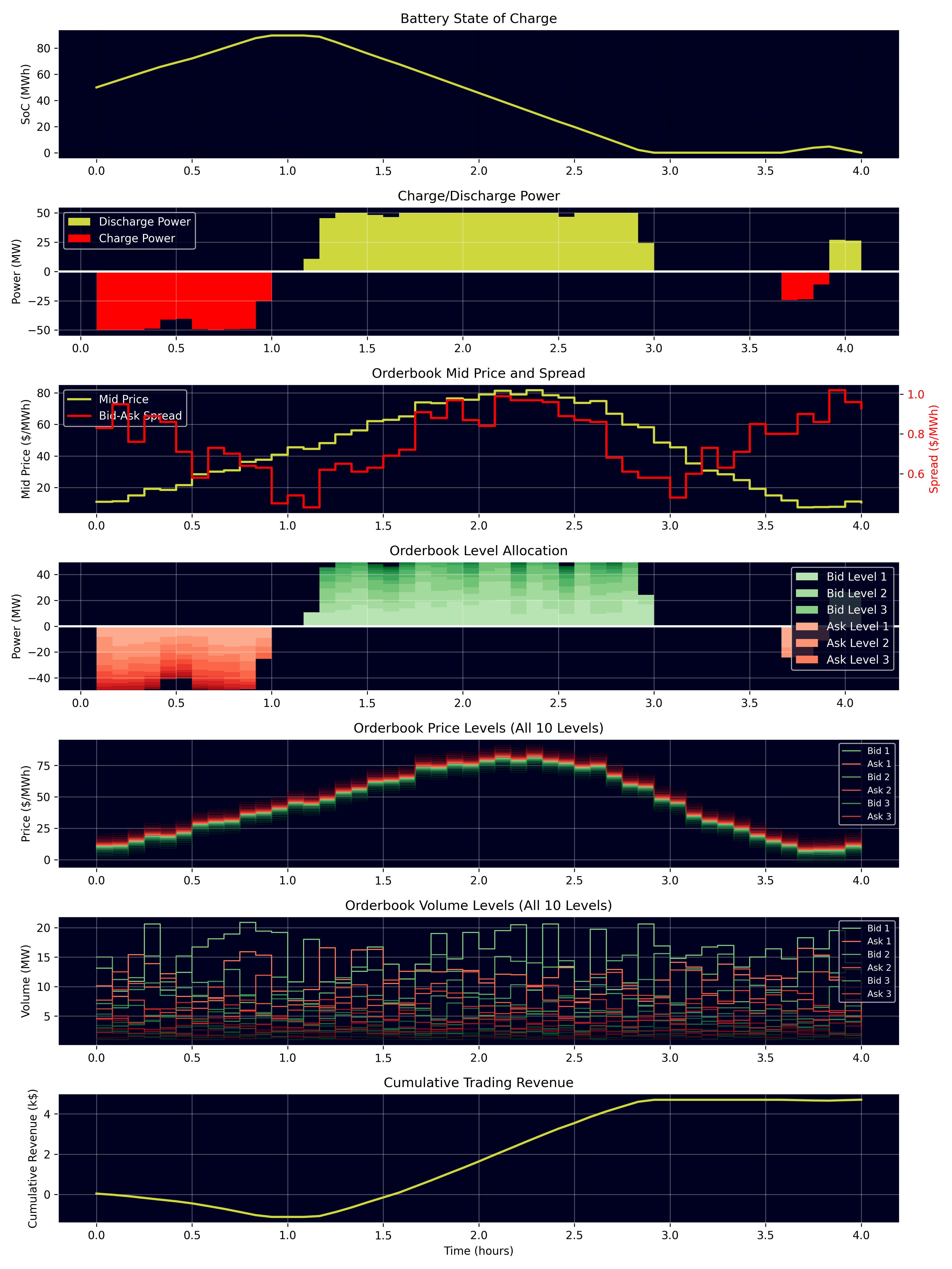
Figure: BESS intraday trading results showing (top to bottom): State of Charge profile, Charge/Discharge power decisions, Orderbook mid price and bid-ask spread, Power allocation across orderbook levels, All orderbook price levels, All orderbook volume levels, and Cumulative trading revenue.

The rolling intrinsic policy enables the battery to:

React to real-time orderbook conditions
Optimize across multiple price levels
Account for liquidity constraints at each level
Maximize trading profit while respecting volume limits