Scheduling Demo: Energy Time Arbitrage

Introduction

This example demonstrates how to use RTC-Tools to optimise a Battery Energy Storage System (BESS) for day-ahead time arbitrage. The optimisation maximizes revenue by strategically charging during low electricity price periods and discharging during high price periods, while accounting for round-trip efficiency losses and cycling penalties.

Market Applicability

This model is applicable to multiple electricity markets:

European Day-Ahead Markets

Optimises for EPEX SPOT and other European day-ahead auctions
Typically 24-hour horizon with hourly resolution

Australian National Electricity Market (NEM)

Optimises for NEM dispatch intervals (5-minute settlement)
Accommodates NEM’s 5-minute dispatch cycles and price volatility

The model is market-agnostic and can be adapted to any day-ahead or dispatch market by adjusting the time series resolution and price data inputs.

Problem Formulation

Mathematical Model

The BESS optimisation problem can be formulated as follows:

Objective Function:

\[\max \sum_{t} \left( P_{net}(t) \cdot \pi(t) - \lambda \cdot (P_{charge}(t) + P_{discharge}(t)) \right)\]

Where:

\(P_{net}(t) = P_{discharge}(t) - P_{charge}(t)\) = Net power (positive for discharge, negative for charge)
\(\pi(t)\) = Electricity price at time t
\(\lambda\) = Cycling penalty factor (requires tuning based on market conditions; annual revision is a reasonable starting point)
\(P_{charge}(t)\) = Charging power
\(P_{discharge}(t)\) = Discharging power

State of Charge Dynamics:

\[3600 \cdot \frac{dSoC}{dt} = P_{charge}(t) \cdot \sqrt{\eta} - \frac{P_{discharge}(t)}{\sqrt{\eta}}\]

Where:

\(SoC\) = State of charge in MWh
\(\eta\) = Round-trip efficiency
The factor 3600 converts from MJ to MWh (seconds to hours)

Variable Bounds:

\[0 \leq SoC(t) \leq 100 \text{ MWh}\]

\[0 \leq P_{charge}(t) \leq 50 \text{ MW}\]

\[0 \leq P_{discharge}(t) \leq 50 \text{ MW}\]

Complementarity Constraints:

The complementarity between charging and discharging is enforced using binary variables and inequality constraints:

\[b_{charge}(t) + b_{discharge}(t) \leq 1\]

\[P_{charge}(t) \leq b_{charge}(t) \cdot P_{max}\]

\[P_{discharge}(t) \leq b_{discharge}(t) \cdot P_{max}\]

Where:

\(b_{charge}(t)\) and \(b_{discharge}(t)\) are binary variables
\(P_{max} = 50\) MW is the maximum power rating

Model Implementation

Architecture Overview

The BESS optimisation follows a clear separation of concerns:

Physical Asset Model (Modelica)

The Modelica model (BESS.mo) focuses purely on the physical behavior of the battery system:

State of charge dynamics with efficiency losses
Power flow calculations
Physical constraints and bounds
No economic calculations

Value Stream Model (Python)

The Python implementation (bess.py) handles all economic aspects:

Revenue calculations from energy arbitrage
Cycling penalty costs
Objective function formulation
Economic parameters and constraints

Physical Asset Model (Modelica)

The BESS physical model is implemented in pure Modelica without external library dependencies:

BESS.mo - Physical asset model (battery dynamics only)

model BESS
  // Parameters
  parameter Real capacity = 100.0 "Battery capacity in MWh";
  parameter Real efficiency = 0.9 "Round-trip efficiency";
  parameter Real max_power = 50.0 "Maximum charge/discharge power in MW";
  
  // Variables
  output Real soc(start=50.0, min=0.0, max=capacity) "State of charge in MWh";
  output Real charge_power(min=0.0, max=max_power) "Charging power in MW";
  output Real discharge_power(min=0.0, max=max_power) "Discharging power in MW";
  output Real net_power "Net power (positive = discharge, negative = charge) in MW";
  
  // Binary variables for complementarity
  Boolean is_charging "True if battery is charging";
  Boolean is_discharging "True if battery is discharging";
  
  // Input variables
  input Real price(fixed = true) "Electricity price in $/MWh";
  
equation
  // State of charge dynamics
  3600 * der(soc) = charge_power * sqrt(efficiency) - discharge_power / sqrt(efficiency);
  
  // Net power calculation
  net_power = discharge_power - charge_power;
  
end BESS;

Value Stream Model (Python)

Objective Function (Economic Model):

    def path_objective(self, ensemble_member):
        """
        Define optimization objective: maximize revenue minus cycling penalty.
        
        This separates the economic value streams (calculated in Python) from
        the physical asset model (defined in Modelica).
        """
        # Revenue from energy arbitrage
        revenue = self.state('net_power') * self.state('price')
        
        # Cycling penalty based on total power throughput
        cycling_penalty = self.cycling_penalty_factor * (
            self.state('charge_power') + self.state('discharge_power')
        )
        
        # Total objective (negative because we want to maximize)
        return -(revenue - cycling_penalty)

The objective function demonstrates the value stream modeling:

Revenue Stream: net_power * price - income from energy arbitrage
Cost Stream: cycling_penalty_factor * (charge_power + discharge_power) - operational costs
Optimization Goal: Maximize net profit (revenue minus costs)

Solver Configuration:

    def solver_options(self):
        """Configure solver options for mixed-integer optimization."""
        options = super().solver_options()
        options['casadi_solver'] = 'qpsol'
        options['solver'] = 'highs'
        return options

The example uses the HiGHS mixed-integer linear programming solver.

Path Constraints:

    def path_constraints(self, ensemble_member):
        """Define path constraints (inequality constraints over time)."""
        constraints = super().path_constraints(ensemble_member)

        parameters = self.parameters(ensemble_member)
        
        # Ensure only one mode can be active at a time (complementarity)
        constraints.append((
            self.state('is_charging') + 
            self.state('is_discharging'),
            -np.inf,
            1.0,
        ))
        constraints.append((
            self.state('charge_power') -
            self.state('is_charging') * parameters["max_power"],
            -np.inf,
            0,
        ))
        constraints.append((
            self.state('discharge_power') -
            self.state('is_discharging') * parameters["max_power"],
            -np.inf,
            0,
        ))
        
        return constraints

The path constraints implement complementarity between charging and discharging.

Input Data

The example uses two CSV input files:

timeseries_import.csv: Contains electricity price forecasts.
initial_state.csv: Specifies the initial state of charge.

Running the Example

Install Dependencies:
```
uv sync
```
Navigate to the Example Directory:
```
cd scheduling
```
Run the Optimization:
```
uv run python src/bess.py
```
This will: * Solve the optimisation problem * Export results to output/timeseries_export.csv
Generate Plots and Summary:
```
uv run python src/plot_results.py
```
This will:
- Read the exported CSV results
- Calculate economic metrics (revenue, costs)
- Generate visualization plots
- Display summary statistics
- Save plots to output/bess_optimisation_results.png

Alternative: Run Both Steps Together:

uv run python src/bess.py && uv run python src/plot_results.py

Results and Analysis

Key outputs from the optimization are visualized below:

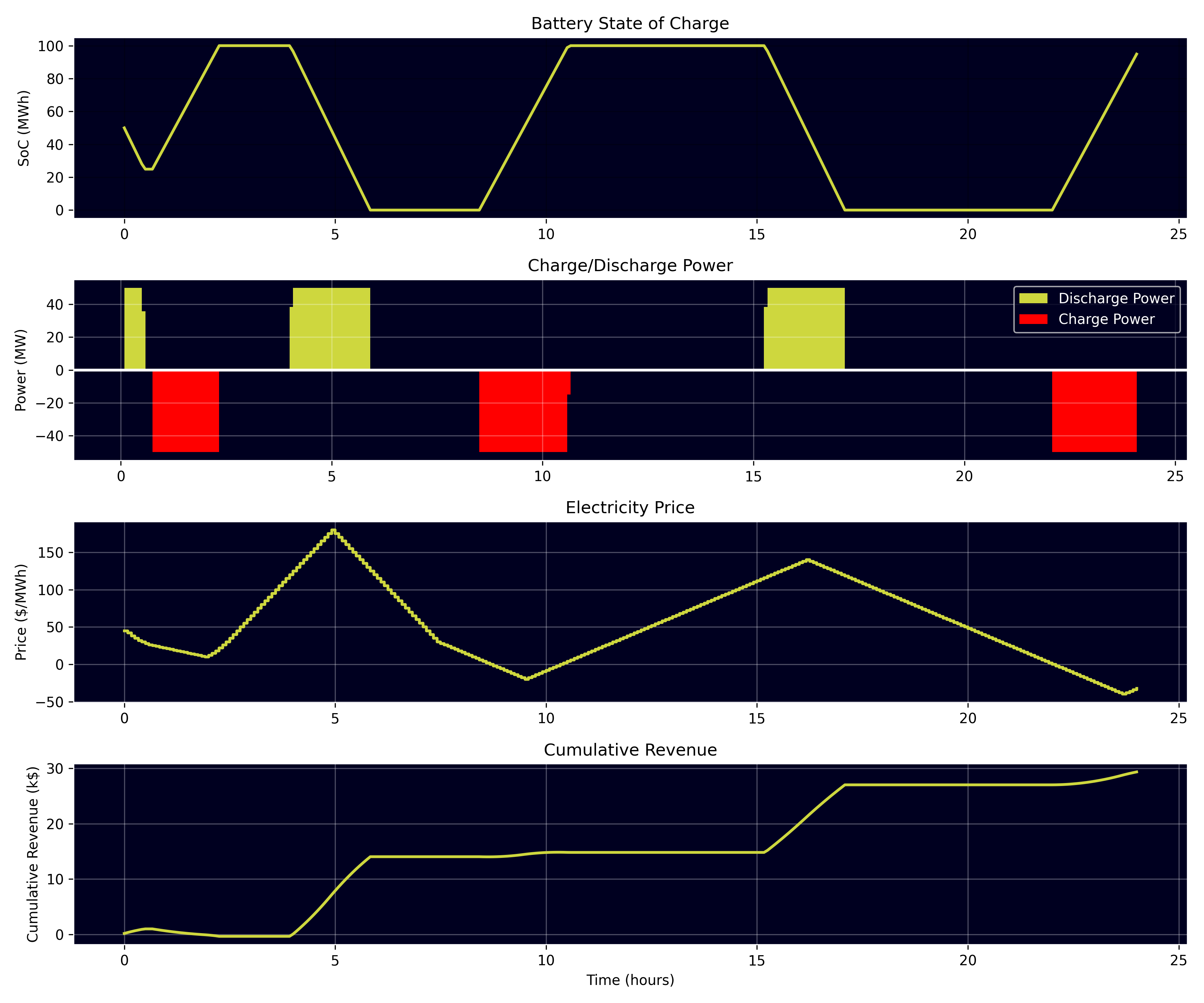
Figure: BESS optimisation results showing (top to bottom): State of Charge profile, Charge/Discharge power decisions, Electricity price signal, and Cumulative revenue over the 24-hour optimisation horizon.